
Súbor:VFPt dipoles electric.svg

Pôvodný súbor (SVG súbor, 840 × 840 pixelov, veľkosť súboru: 108 KB)
Zhrnutie
| Popis |
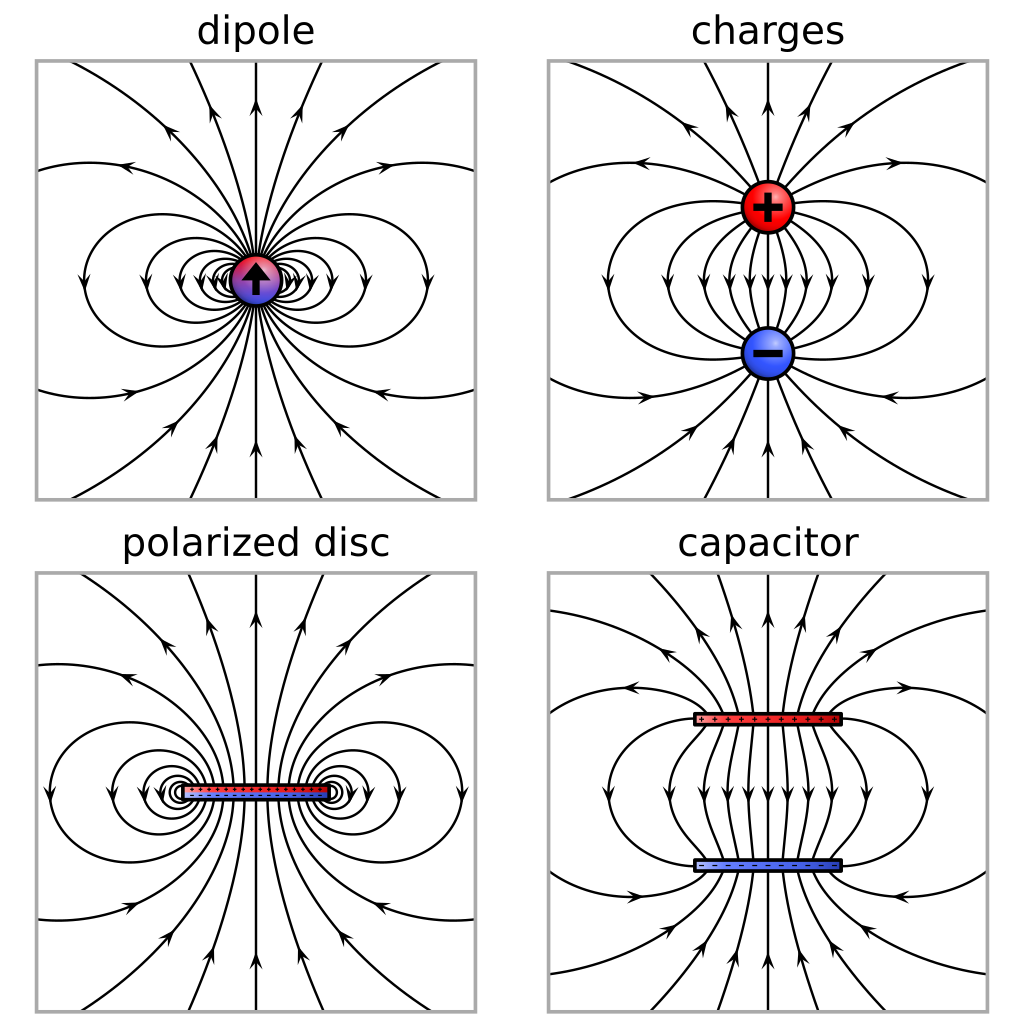
English: Computed drawings of four different types of electric dipoles.
Upper left: An ideal point-like dipole. The field shape is scale invariant and approximates the field of any charge configuration with nonzero dipole moment at large distance. Русский: Рассчитанные электростатические поля четырех различных типов электрических диполей.
Поле идеального точечного диполя. Конфигурация поля в большом масштабе инвариантна и приблизительно соответствует полю любой конфигурации зарядов с ненулевым дипольным моментом на большом расстоянии. Дискретный диполь двух противоположных точечных зарядов разнесенных на конечное расстояние, – физический диполь. Тонкий круглый диск с равномерной электрической поляризацией вдоль оси симметрии. Плоский конденсатор с одинаково заряженными круглыми обкладками. Несмотря на различие этих конфигураций, вблизи которых поля существенно различаются, все эти поля сходятся к одному и тому же дипольному полю на больших расстояниях где они приблизительно одинаковы, при этом любая система зарядов может моделировать идеальный электрический диполь. |
| Dátum | |
| Zdroj | Vlastné dielo |
| Autor | Geek3 |
| Ďalšie verzie |
|
| SVG vývoj | Táto grafika bola vytvorená pomocou VectorFieldPlot. This file is translated using SVG switch elements: all translations are stored in the same file. |
| Zdrojový kód | Python code# paste this code at the end of VectorFieldPlot 3.3
R = 0.6
h = 0.6
rsym = 21
doc = FieldplotDocument('VFPt_dipoles_electric1', commons=True,
width=360, height=360)
field = Field([ ['dipole', {'x':0, 'y':0, 'px':0., 'py':1.}] ])
def f_arrows(xy):
return xy[1] * (sc.hypot(xy[0], xy[1]) / 1.4 - 1)
def f_cond(xy):
return hypot(*xy) > 1e-4 and (fabs(xy[1]) < 1e-3 or fabs(xy[1]) > .3)
nlines = 19
startpoints = Startpath(field, lambda t: 0.25*sc.array([sin(t), cos(t)]),
t0=-pi/2, t1=pi/2).npoints(nlines)
for p0 in startpoints:
line = FieldLine(field, p0, directions='both')
doc.draw_line(line, maxdist=1, arrows_style={'at_potentials':[0.],
'potential':f_arrows, 'condition_func':f_cond, 'scale':1.2})
# draw dipole symbol
rb_grad = etree.SubElement(doc._get_defs(), 'linearGradient')
rb_grad.set('id', 'grad_rb')
for attr, val in [['x1', '0'], ['x2', '0'], ['y1', '0'], ['y2', '1']]:
rb_grad.set(attr, val)
for col, of in [['#3355ff', '0'], ['#9944aa', '0.5'], ['#ff0000', '1']]:
stop = etree.SubElement(rb_grad, 'stop')
stop.set('stop-color', col)
stop.set('offset', of)
stop.set('stop-opacity', '1')
symb = doc.draw_object('g', {'id':'dipole_symbol',
'transform':'scale({0},{0})'.format(1./doc.unit)})
doc.draw_object('circle', {'cx':'0', 'cy':'0', 'r':rsym,
'fill':'url(#grad_rb)', 'stroke':'none'}, group=symb)
doc._check_whitespot()
doc.draw_object('circle', {'cx':'0', 'cy':'0', 'r':rsym,
'fill':'url(#white_spot)', 'stroke':'#000000', 'stroke-width':'3'},
group=symb)
doc.draw_object('path', {'fill':'#000000', 'stroke':'none',
'd':'M 3,-12 V 0 H 12 L 0,15 L -12,0 H -3 V -12 H 3 Z'}, group=symb)
doc.write()
doc = FieldplotDocument('VFPt_dipoles_electric2', commons=True,
width=360, height=360)
field = Field([ ['monopole', {'x':0, 'y':h, 'Q':1}],
['monopole', {'x':0, 'y':-h, 'Q':-1}] ])
def f_arrows(xy):
return xy[1] * (sc.hypot(xy[0], xy[1]) / 1.4 - 1)
def f_cond(xy):
return fabs(xy[0]) < 1.4
nlines = 18
stp = Startpath(field, lambda t: R*sc.array([.2*sin(t), 1+.2*cos(t)]),
t0=-pi, t1=pi)
startpoints = [stp.startpos(s) for s in sc.arange(nlines)/float(nlines)]
startpoints.append(startpoints[nlines//2].dot([[1,0],[0,-1]]))
for p0 in startpoints:
line = FieldLine(field, p0, directions='both', maxr=100)
doc.draw_line(line, maxdist=1, arrows_style={'at_potentials':[0.],
'potential':f_arrows, 'condition_func':f_cond, 'scale':1.2})
# draw charge symbols
symb_plus = doc.draw_object('g', {
'transform':'translate(0,{0}) scale({1},{1})'.format(h, 1./doc.unit)})
symb_minus = doc.draw_object('g', {
'transform':'translate(0,{0}) scale({1},{1})'.format(-h, 1./doc.unit)})
for i, g in enumerate([symb_plus, symb_minus]):
doc.draw_object('circle', {'cx':'0', 'cy':'0', 'r':rsym, 'stroke':'none',
'fill':['#ff0000', '#3355ff'][i]}, group=g)
doc._check_whitespot()
doc.draw_object('circle', {'cx':'0', 'cy':'0', 'r':rsym,
'fill':'url(#white_spot)', 'stroke':'#000000', 'stroke-width':'3'}, group=g)
c_symb = doc.draw_object('path', {'fill':'#000000', 'stroke':'none'}, group=g)
if i == 0: # plus sign
c_symb.set('d', 'M 3,3 V 12 H -3 V 3 H -12 V -3'
+ ' H -3 V -12 H 3 V -3 H 12 V 3 H 3 Z')
else: # minus sign
c_symb.set('d', 'M 12,3 H -12 V -3 H 12 V 3 Z')
doc.write()
doc = FieldplotDocument('VFPt_dipoles_electric3', commons=True,
width=360, height=360)
field = Field([ ['ringcurrent', {'x':0, 'y':0, 'R':R, 'phi':pi/2, 'I':1.}] ])
def f_arrows(xy):
return xy[1] * (sc.hypot(xy[0], xy[1]) / 1.4 - 1)
def f_cond(xy):
return hypot(*xy) > 1.2*R and fabs(fabs(xy[0]) - 1.4) > 0.2
nlines = 19
startpoints = Startpath(field, lambda t: sc.array([R*t, 0.]),
t0=-0.9375, t1=0.9375).npoints(nlines)
for p0 in startpoints:
line = FieldLine(field, p0, directions='both')
doc.draw_line(line, maxdist=1, arrows_style={'at_potentials':[0.],
'potential':f_arrows, 'condition_func':f_cond, 'scale':1.2})
# draw polarized sheet
sheet = doc.draw_object('g', {'id':'polarized_sheet'})
s = 0.06
doc.draw_object('rect', {'x':-R, 'y':-s, 'width':2*R, 'height':2*s,
'stroke':'none', 'fill':'#3355ff'}, group=sheet)
doc.draw_object('rect', {'x':-R, 'y':0, 'width':2*R, 'height':s,
'stroke':'none', 'fill':'#ff0000'}, group=sheet)
grad = doc.draw_object('linearGradient', {'id':'grad-round',
'x1':str(R), 'x2':str(-R), 'y1':'0', 'y2':'0',
'gradientUnits':'userSpaceOnUse'}, group=doc.defs)
for o, c, a in ((0, '#000', 0.3), (0.3, '#999', 0.2),
(0.8, '#fff', 0.25), (1, '#fff', 0.65)):
doc.draw_object('stop', {'id':'grad',
'offset':str(o), 'stop-color':c, 'stop-opacity':str(a)}, grad)
doc.draw_object('rect', {'x':-R, 'y':-s, 'width':2*R, 'height':2*s,
'stroke':'#000000', 'stroke-width':0.03, 'fill':'url(#grad-round)',
'stroke-linejoin':'round'}, group=sheet)
symbols_plus = []
symbols_minus = []
for x in sc.linspace(-R*0.875, R*0.875, 16):
symbols_minus.append('M {:.3f},0 h 0.03'.format(x-0.015))
symbols_plus.append('M {:.3f},0 h 0.03 M {:.3f},-0.015 v 0.03'.format(
x-0.015, x))
doc.draw_object('path', {'d':' '.join(symbols_plus), 'stroke':'#000000',
'fill':'none', 'stroke-width':0.01, 'stroke-linecap':'butt',
'transform':'translate(0,0.025)'}, group=sheet)
doc.draw_object('path', {'d':' '.join(symbols_minus), 'stroke':'#000000',
'fill':'none', 'stroke-width':0.01, 'stroke-linecap':'butt',
'transform':'translate(0,-0.025)'}, group=sheet)
doc.write()
doc = FieldplotDocument('VFPt_dipoles_electric4', commons=True,
width=360, height=360)
field_D = Field([ ['coil', {'x':0, 'y':0, 'phi':pi/2, 'R':R, 'Lhalf':h,
'I':1./(R**2*pi)}] ])
field_E = Field([ ['charged_disc', {'x0':-R, 'x1':R, 'y0':h, 'y1':h, 'Q':.5/h}],
['charged_disc', {'x0':-R, 'x1':R, 'y0':-h, 'y1':-h, 'Q':-.5/h}] ])
field_E_inside = Field([ ['homogeneous', {'Fx':0., 'Fy':-.5/(h*R**2*pi)}],
['coil', {'x':0, 'y':0, 'phi':pi/2, 'R':R, 'Lhalf':h, 'I':1./(R**2*pi)}] ])
def f_arrows(xy):
return xy[1] * (sc.hypot(xy[0], xy[1]) / 1.4 - 1)
def f_cond(xy):
return True
# Use fieldlines in D-field to find good starting points
nlines = 13
startpoints = []
startpoints2 = []
for iline in range(nlines):
p0 = sc.array([R * (-1. + 2. * (iline + 0.5) / nlines), 0.])
print('p0', p0)
line_D = FieldLine(field_D, p0, directions='forward',
maxr=100, stop_funcs=2*[lambda xy: -xy[1] - max(0, 1-hypot(*xy)/R)])
p1 = line_D.nodes[-1]['p']
startpoints.append(p1)
if iline >= 3 and iline < nlines - 3:
line_D = FieldLine(field_D, p0, directions='forward',
maxr=2, stop_funcs=2*[lambda xy: xy[1] - h])
p2 = line_D.nodes[-1]['p']
startpoints2.append(p2)
startpoints.append([0, -3])
for p0 in startpoints:
line = FieldLine(field_E, p0, directions='both', maxr=100)
doc.draw_line(line, maxdist=1, arrows_style={'at_potentials':[0.],
'potential':f_arrows, 'condition_func':f_cond, 'scale':1.2})
for p0 in startpoints2:
line = FieldLine(field_E_inside, p0, directions='forward',
stop_funcs=2*[lambda xy: -xy[1] - h])
doc.draw_line(line, maxdist=1, arrows_style={'at_potentials':[0.],
'potential':f_arrows, 'condition_func':f_cond, 'scale':1.2})
# draw charged discs
disc_plus = doc.draw_object('g', {'id':'disc_plus',
'transform':'translate(0,{0})'.format(h)})
disc_minus = doc.draw_object('g', {'id':'disc_minus',
'transform':'translate(0,{0})'.format(-h)})
s = 0.045
grad = doc.draw_object('linearGradient', {'id':'grad-round',
'x1':str(R), 'x2':str(-R), 'y1':'0', 'y2':'0',
'gradientUnits':'userSpaceOnUse'}, group=doc.defs)
for o, c, a in ((0, '#000', 0.3), (0.3, '#999', 0.2),
(0.8, '#fff', 0.25), (1, '#fff', 0.65)):
doc.draw_object('stop', {
'offset':str(o), 'stop-color':c, 'stop-opacity':str(a)}, grad)
for i, g in enumerate([disc_plus, disc_minus]):
doc.draw_object('rect', {'x':-R, 'y':-s, 'width':2*R, 'height':2*s,
'stroke':'none', 'fill':['#ff0000', '#3355ff'][i]}, group=g)
doc.draw_object('rect', {'x':-R, 'y':-s, 'width':2*R, 'height':2*s,
'stroke':'#000000', 'stroke-width':0.03, 'fill':'url(#grad-round)',
'stroke-linejoin':'round'}, group=g)
symbols = []
for x in [R * (2 * (0.5 + isy) / 11 - 1) for isy in range(11)]:
if i == 0:
d = 'M {:.3f},0 h 0.04 M {:.3f},-0.02 v 0.04'.format(x-0.02, x)
else:
d = 'M {:.3f},0 h 0.04'.format(x-0.02)
symbols.append(d)
doc.draw_object('path', {'d':' '.join(symbols), 'stroke':'#000000',
'fill':'none', 'stroke-width':0.01, 'stroke-linecap':'butt'}, group=g)
doc.write()
|


Licencovanie
- Môžete slobodne:
- zdieľať – kopírovať, šíriť a prenášať dielo
- meniť ho – upravovať dielo
- Za nasledovných podmienok:
- uvedenie autorov – Musíte spomenúť autorov (jednotlivo alebo kolektívne), poskytnúť odkaz na licenciu a uviesť, či ste niečo zmenili. Môžete to urobiť ľubovoľným primeraným spôsobom, ale nie spôsobom naznačujúcim, že poskytovateľ licencie podporuje vás alebo vaše použitie diela.
- meniť za rovnakých podmienok – Ak toto dielo zmeníte, prevediete do inej formy alebo použijete ako základ iného diela, musíte výsledok šíriť pod rovnakou alebo kompatibilnou licenciou ako originál.
História súboru
Po kliknutí na dátum/čas uvidíte ako súbor vyzeral vtedy.
| Dátum/Čas | Náhľad | Rozmery | Používateľ | Komentár | |
|---|---|---|---|---|---|
| aktuálna | 21:37, 22. máj 2021 | | 840 × 840 (108 KB) | Geek3 | added russion captions from VFPt_dipoles_electric-ru.svg |
| 16:25, 11. január 2020 |  | 840 × 840 (107 KB) | Geek3 | User created page with UploadWizard |
Použitie súboru
Na tento súbor odkazuje nasledujúca stránka:
Globálne využitie súborov
Nasledovné ďalšie wiki používajú tento súbor:
- Použitie na bn.wikipedia.org
- Použitie na en.wikipedia.org